Optimization & MCDA — Weighted Scoring, Quick LP

Security teams face a recurring problem: too many candidate controls, not enough budget, and no principled way to rank them. Stakeholders want to know why a particular control was selected over another, so the ranking method must be explainable.

These are not theoretical exercises. Every annual security budget cycle involves exactly this problem: a list of initiatives competing for limited funds, each championed by a different team, each claiming to be critical. Without a structured framework, the loudest voice or the most recent incident wins. MCDA and optimization provide an alternative grounded in explicit criteria and reproducible logic.

A typical security roadmap might list 15–20 candidate initiatives: endpoint detection, MFA expansion, network segmentation, backup hardening, security awareness training, cloud posture management, and so on. Each costs a different amount, reduces different risks by different degrees, takes a different amount of time to implement, and requires different skills. Choosing the best subset under a fixed budget is a combinatorial problem, and intuition alone handles it poorly once you pass five or six options.

This notebook walks through three complementary approaches:

1. Multi-Criteria Decision Analysis (MCDA) — weighted scoring across several criteria, with a sensitivity check on the weights.

2. Greedy ROI selection — pick controls in decreasing bang-for-buck order until the budget runs out.

3. Linear Programming (LP) — the relaxed 0-1 knapsack, which gives an upper bound on what any feasible selection can achieve.

What all three methods share is transparency. The inputs (scores, weights, costs, risk-reduction estimates) are visible and debatable. The logic is reproducible. And the outputs can be stress-tested by varying assumptions. This stands in sharp contrast to the more common approach: a senior leader ranks controls by gut feel in a spreadsheet, and everyone else reverse-engineers the rationale after the fact.

Each method answers a slightly different question. Understanding when they agree — and when they disagree — is the real takeaway.

Decision-Theoretic Foundations

The weighted scoring approach in this notebook has deep roots in formal decision theory — specifically, multiattribute utility theory developed by Raiffa (1968) and Keeney and Raiffa (1976). Understanding these foundations is not required to use MCDA, but it explains why the method works and when it breaks down.

When a decision involves multiple attributes — cost, risk reduction, implementation time, compliance alignment — the question is not whether to weight them, but whether to weight them explicitly or implicitly. Every control selection involves multi-attribute trade-offs. When a CISO says “EDR is more important than SIEM,” they have already assigned weights — they just haven’t written them down.

Raiffa showed that if a decision-maker’s preferences satisfy two behavioral axioms, then there exists a utility function that represents those preferences as a weighted sum over attribute scores:

\[u(C) = \sum_k w_k \, u_k(x_k)\]

Two key axioms (Raiffa 1968; Keeney & Raiffa 1976):

1. Transitivity: If you prefer A to B and B to C, you must prefer A to C. Violations create “money pumps” — circular preferences that vendors can exploit (see notebook 05).

2. Substitutability: If you are indifferent between two prizes in a lottery, swapping one for the other should not change your preference. This lets us replace complex multi-attribute outcomes with single-number scores.

This result is significant because it means the MCDA approach in this notebook is not an arbitrary heuristic. When the axioms hold, weighted scoring is the unique representation consistent with the decision-maker’s preferences. The weights encode the relative importance of each criterion, and the normalization ensures commensurability across scales.

The axioms also reveal where MCDA can mislead:

• Transitivity violations (discussed in Chapter 0.5 under intransitive preferences) mean the decision-maker’s implicit preferences cannot be represented by any set of consistent weights. The right response is to resolve the intransitivity before scoring, not to force a weighting that papers over the inconsistency.

• Substitutability failures occur when attributes interact — for example, when the value of compliance alignment depends on the level of risk reduction already achieved. These cases require more sophisticated models (multiplicative utility) that go beyond the additive form used here.

For most security control-selection problems, the additive model is a reasonable starting point. The key insight from Raiffa is that weighted scoring is not merely a convenient tool — it is the minimum formal structure needed to make multi-criteria decisions consistently, and its limitations are precisely the limitations of the underlying preference axioms.

The practical message: MCDA is not an arbitrary scoring exercise. It is the simplest formal model that is consistent with rational multi-attribute preferences. The weights are the hard part — not because the math demands them, but because they force explicit trade-offs that organizations normally leave implicit.

1 — Setup

We use decision-security’s ROI selector, pandas for tabular data, scipy’s linear programming solver, and matplotlib for visualization.

import numpy as np
import pandas as pd
import matplotlib.pyplot as plt
from scipy.optimize import linprog

from decision_security.synth import make_rng
from decision_security.voi import select_controls_by_roi

rng = make_rng(42)
plt.rcParams.update({
    "font.family": "serif",
    "font.size": 10,
    "axes.labelsize": 11,
    "axes.titlesize": 12,
    "xtick.labelsize": 9,
    "ytick.labelsize": 9,
    "legend.fontsize": 9,
    "figure.dpi": 150,
    "axes.spines.top": False,
    "axes.spines.right": False,
})

PRIMARY = "#1A1A1A"
ACCENT = "#E74C3C"
DARK_BG = "#34495E"
LIGHT_GRAY = "#95A5A6"
MED_GRAY = "#7F8C8D"
VERY_LIGHT = "#BDC3C7"

2 — MCDA: Weighted Scoring

Multi-criteria decision analysis scores each candidate control across several dimensions — risk reduction, implementation cost, time to deploy, operational complexity, regulatory alignment — then combines them into a single weighted score:

\[\text{score}_i = \sum_k w_k \cdot s_{ik}\]

where \(w_k\) are the criteria weights (summing to 1) and \(s_{ik}\) is the normalized score of control \(i\) on criterion \(k\).

Normalization matters. Raw scores on different scales (dollars, months, percentage risk reduction) must be mapped to a common range, typically \([0, 1]\), before weighting. Min-max normalization is the simplest approach:

\[s_{ik} = \frac{x_{ik} - \min_k}{\max_k - \min_k}\]

The choice of normalization method can change rankings — this is not a bug but a feature, because it forces you to decide what “better” means on each dimension.

We evaluate six candidate controls against four criteria. Three of the criteria are “inverse” (lower raw value is better), so we name them with an _inv suffix and flip them before scoring.

Criterion	Weight	Direction
risk_reduction	0.40	higher is better
cost_inv	0.30	lower cost is better
time_inv	0.15	shorter implementation is better
complexity_inv	0.15	simpler is better

The weights encode stakeholder priorities. A CISO focused on regulatory deadlines might weight compliance alignment heavily; a CTO focused on operational stability might weight implementation complexity. Making weights explicit and visible is the primary benefit of MCDA — it transforms “I just think MFA is more important” into a testable, debatable parameter.

Tip: A practical approach to weight elicitation: ask each stakeholder to distribute 100 points across the criteria. Average the distributions, then show individual allocations alongside the average. Disagreements about weights are often more informative than the final ranking — they reveal where the leadership team lacks alignment on strategic priorities.

controls = [
    "MFA Rollout",
    "EDR Deployment",
    "Network Segmentation",
    "Security Awareness",
    "Patch Automation",
    "DLP Gateway",
]

# Raw scores — higher is better for risk_reduction;
# lower is better for cost, time, complexity.
raw = pd.DataFrame(
    {
        "risk_reduction": [0.35, 0.50, 0.45, 0.15, 0.40, 0.25],
        "cost_inv":       [50, 200, 180, 30, 90, 150],       # $K
        "time_inv":       [2, 6, 8, 1, 3, 5],                # months
        "complexity_inv": [2, 4, 5, 1, 3, 4],                # 1-5 scale
    },
    index=controls,
)
raw

	risk_reduction	cost_inv	time_inv	complexity_inv
MFA Rollout	0.35	50	2	2
EDR Deployment	0.50	200	6	4
Network Segmentation	0.45	180	8	5
Security Awareness	0.15	30	1	1
Patch Automation	0.40	90	3	3
DLP Gateway	0.25	150	5	4

def normalize_mcda(df):
    """Min-max normalise each column to [0, 1].
    Columns ending in '_inv' are flipped so that lower raw = higher score."""
    normed = pd.DataFrame(index=df.index)
    for col in df.columns:
        lo, hi = df[col].min(), df[col].max()
        span = hi - lo if hi != lo else 1.0
        if col.endswith("_inv"):
            normed[col] = (hi - df[col]) / span
        else:
            normed[col] = (df[col] - lo) / span
    return normed


normed = normalize_mcda(raw)
normed.round(3)

	risk_reduction	cost_inv	time_inv	complexity_inv
MFA Rollout	0.571	0.882	0.857	0.75
EDR Deployment	1.000	0.000	0.286	0.25
Network Segmentation	0.857	0.118	0.000	0.00
Security Awareness	0.000	1.000	1.000	1.00
Patch Automation	0.714	0.647	0.714	0.50
DLP Gateway	0.286	0.294	0.429	0.25

weights = np.array([0.40, 0.30, 0.15, 0.15])
assert np.isclose(weights.sum(), 1.0), "Weights must sum to 1"

normed["weighted_score"] = normed.values @ weights
normed["rank"] = normed["weighted_score"].rank(ascending=False).astype(int)
normed.sort_values("rank")

	risk_reduction	cost_inv	time_inv	complexity_inv	weighted_score	rank
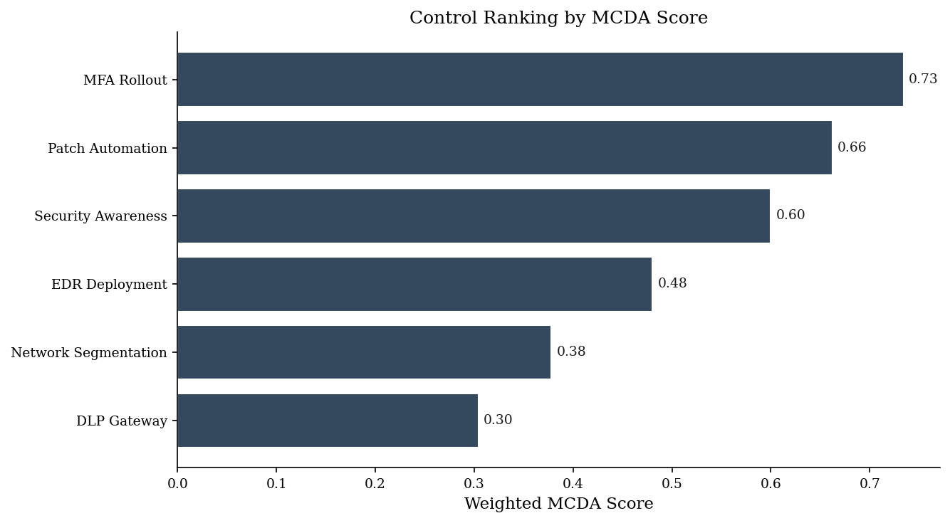
MFA Rollout	0.571429	0.882353	0.857143	0.75	0.734349	1
Patch Automation	0.714286	0.647059	0.714286	0.50	0.661975	2
Security Awareness	0.000000	1.000000	1.000000	1.00	0.600000	3
EDR Deployment	1.000000	0.000000	0.285714	0.25	0.480357	4
Network Segmentation	0.857143	0.117647	0.000000	0.00	0.378151	5
DLP Gateway	0.285714	0.294118	0.428571	0.25	0.304307	6

sorted_df = normed.sort_values('weighted_score', ascending=True)
fig, ax = plt.subplots(figsize=(9, 5))
ax.barh(sorted_df.index, sorted_df['weighted_score'], color=DARK_BG, edgecolor='white')
for i, (idx_name, row) in enumerate(sorted_df.iterrows()):
    ax.text(row['weighted_score'] + 0.005, i, f'{row["weighted_score"]:.2f}',
            va='center', fontsize=9, color=PRIMARY)
ax.set_xlabel('Weighted MCDA Score')
ax.set_title('Control Ranking by MCDA Score')
plt.tight_layout()
plt.show()

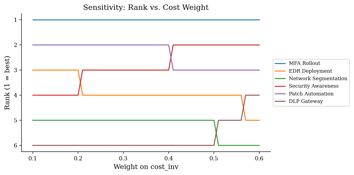
3 — Sensitivity Analysis

Any ranking that depends on weights should be stress-tested. Sensitivity analysis asks: how much would a weight need to change before the top-ranked control loses its position? These critical thresholds are called flip points, and they reveal whether a ranking is robust or fragile.

If swinging the cost weight from 0.25 to 0.30 flips the top two controls, the ranking is sensitive and the weight choice deserves more scrutiny. If the top control dominates across all plausible weight ranges, you can proceed with confidence.

We vary the cost_inv weight from 0.10 to 0.60, redistributing the remaining weight among the other three criteria in the same proportions they had originally. The code identifies exact flip points where rank swaps occur.

In practice, presenting sensitivity results to stakeholders is as valuable as the ranking itself. When a decision-maker sees that their preferred control only wins under a narrow weight range, the conversation shifts from “which control is best?” to “how much do we actually value this criterion?” — which is the right question to be asking.

base_weights = np.array([0.40, 0.30, 0.15, 0.15])
cost_idx = 1  # cost_inv is the second criterion

cost_range = np.arange(0.10, 0.61, 0.01)
rank_history = {c: [] for c in controls}

for cw in cost_range:
    w = base_weights.copy()
    remaining = 1.0 - cw
    others_sum = base_weights.sum() - base_weights[cost_idx]
    for j in range(len(w)):
        if j == cost_idx:
            w[j] = cw
        else:
            w[j] = base_weights[j] / others_sum * remaining
    scores = normalize_mcda(raw).values @ w
    order = (-scores).argsort()
    ranks = np.empty_like(order)
    ranks[order] = np.arange(1, len(order) + 1)
    for i, c in enumerate(controls):
        rank_history[c].append(ranks[i])

fig, ax = plt.subplots(figsize=(8, 4))
for c in controls:
    ax.plot(cost_range, rank_history[c], label=c)
ax.set_xlabel("Weight on cost_inv")
ax.set_ylabel("Rank (1 = best)")
ax.set_title("Sensitivity: Rank vs. Cost Weight")
ax.invert_yaxis()
ax.legend(loc="center left", bbox_to_anchor=(1, 0.5), fontsize=8)
plt.tight_layout()
plt.show()

# Identify flip points — cost weights where adjacent ranks swap
print("Flip points (cost_inv weight where a rank swap occurs):")
prev_ranks = {c: rank_history[c][0] for c in controls}
for step, cw in enumerate(cost_range[1:], 1):
    for c in controls:
        if rank_history[c][step] != prev_ranks[c]:
            print(f"  cost_w={cw:.2f}: {c} moved from rank {prev_ranks[c]} to {rank_history[c][step]}")
    prev_ranks = {c: rank_history[c][step] for c in controls}

Flip points (cost_inv weight where a rank swap occurs):
  cost_w=0.21: EDR Deployment moved from rank 3 to 4
  cost_w=0.21: Security Awareness moved from rank 4 to 3
  cost_w=0.41: Security Awareness moved from rank 3 to 2
  cost_w=0.41: Patch Automation moved from rank 2 to 3
  cost_w=0.51: Network Segmentation moved from rank 5 to 6
  cost_w=0.51: DLP Gateway moved from rank 6 to 5
  cost_w=0.57: EDR Deployment moved from rank 4 to 5
  cost_w=0.57: DLP Gateway moved from rank 5 to 4

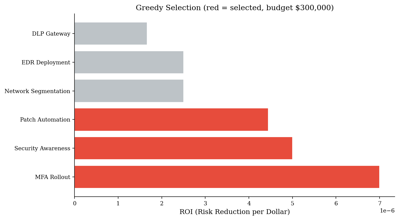
4 — Greedy ROI Selection

When the goal is simply to maximize risk reduction under a budget constraint, a greedy approach is fast and intuitive: compute each control’s risk reduction per dollar (ROI), sort descending, and select controls in order until the budget is exhausted.

This works well when controls are roughly independent and similarly sized. It is the same logic behind the fractional knapsack solution in algorithms courses, and it produces optimal results when items can be partially selected. For indivisible controls (you either deploy MFA or you don’t), greedy is a good heuristic but not guaranteed optimal — though in practice it is usually within a few percent of the true optimum.

Where greedy fails is when a high-ROI but expensive control consumes most of the budget, preventing two medium-ROI controls that together would deliver more total reduction. The classic knapsack counterexample applies directly: sometimes skipping the “best” item and packing two smaller ones yields a better total. We compare greedy output to LP-optimal output below to show when and how much this matters.

We use select_controls_by_roi from decision-security with a $300K budget.

deltas = raw["risk_reduction"].values
costs = raw["cost_inv"].values * 1_000  # convert $K to $
budget = 300_000

chosen_idx, total_cost, total_delta = select_controls_by_roi(deltas, costs, budget)

roi_table = pd.DataFrame(
    {
        "control": [controls[i] for i in chosen_idx],
        "risk_reduction": [deltas[i] for i in chosen_idx],
        "cost_K": [costs[i] / 1_000 for i in chosen_idx],
        "roi": [deltas[i] / costs[i] * 1_000 for i in chosen_idx],
    }
)
roi_table["cumulative_cost_K"] = roi_table["cost_K"].cumsum()
roi_table["cumulative_reduction"] = roi_table["risk_reduction"].cumsum()

print(f"Budget: ${budget:,.0f}")
print(f"Spent:  ${total_cost:,.0f}  |  Risk reduced: {total_delta:.2f}")
roi_table

Budget: $300,000
Spent:  $170,000  |  Risk reduced: 0.90

	control	risk_reduction	cost_K	roi	cumulative_cost_K	cumulative_reduction
0	MFA Rollout	0.35	50.0	0.007000	50.0	0.35
1	Security Awareness	0.15	30.0	0.005000	80.0	0.50
2	Patch Automation	0.40	90.0	0.004444	170.0	0.90

5 — MCDA vs. ROI: When They Disagree

MCDA and greedy ROI can produce different selections because they optimize different objectives. ROI selection optimizes a single dimension — risk reduction per dollar. MCDA balances multiple concerns. When they diverge, it usually means the top-ROI control scores poorly on a dimension that MCDA weights care about (e.g., it is fast and cheap but creates heavy operational burden).

Aspect	MCDA	Greedy ROI
Objective	Highest overall score across criteria	Maximum risk reduction per dollar
Budget awareness	Not inherently budget-constrained	Stops at the budget cap
Criteria breadth	Considers time, complexity, etc.	Only risk reduction and cost
Explainability	Transparent weights; auditable	Simple ratio; easy to verify

Neither method is universally better:

• MCDA when stakeholders care about more than just cost and risk — for example, implementation speed, operational complexity, or regulatory alignment.

• ROI when the decision is purely financial and the single objective is clear: maximize risk reduction subject to a hard budget.

• Both together as a sanity check: if a control ranks highly on MCDA but is absent from the ROI selection, investigate why (often it is expensive relative to its risk reduction alone).

A useful heuristic: if the MCDA ranking and the ROI ranking agree on the top three controls, you have a robust selection regardless of method. If they disagree significantly, the disagreement itself is the most valuable output — it tells you exactly which trade-offs need executive attention rather than analyst judgment.

6 — Linear Programming: Relaxed 0-1 Knapsack

For larger portfolios or tighter constraints, linear programming (LP) provides a rigorous alternative to greedy heuristics. The control selection problem maps directly to a 0-1 knapsack formulation:

\[\max \sum_i v_i \, x_i \quad \text{subject to} \quad \sum_i c_i \, x_i \leq B, \quad x_i \in \{0, 1\}\]

where \(v_i\) is the risk reduction of control \(i\), \(c_i\) is its cost, \(B\) is the total budget, and \(x_i\) indicates whether control \(i\) is selected.

The LP relaxation allows \(x_i\) to take any value in \([0, 1]\), which provides an upper bound on the achievable risk reduction and is solvable in milliseconds. Comparing the relaxed solution to the greedy integer solution tells you how much optimality you are leaving on the table — often very little for security portfolios with moderate numbers of controls.

You can also add side constraints beyond budget: maximum headcount for implementation, minimum coverage of certain risk categories, or mutual exclusivity (choose cloud WAF or on-prem WAF, not both). Each constraint is an additional row in the LP matrix.

scipy.optimize.linprog minimizes, so we negate risk reduction to maximize it.

n = len(controls)

# Objective: minimise -delta (= maximise delta)
c_obj = -deltas

# Constraint: total cost <= budget
A_ub = [costs]           # one row
b_ub = [budget]

# Bounds: 0 <= x_i <= 1  (LP relaxation)
bounds = [(0, 1)] * n

result = linprog(c_obj, A_ub=A_ub, b_ub=b_ub, bounds=bounds, method="highs")
assert result.success, f"LP failed: {result.message}"

lp_reduction = -result.fun
lp_allocation = pd.Series(result.x, index=controls).round(4)

print(f"LP relaxation — max risk reduction: {lp_reduction:.4f}")
print(f"Greedy ROI    — risk reduction:     {total_delta:.4f}")
print(f"Gap:          {lp_reduction - total_delta:.4f}")
print()
print("Allocation (1.0 = fully selected, fractional = partially):")
lp_allocation

LP relaxation — max risk reduction: 1.2250
Greedy ROI    — risk reduction:     0.9000
Gap:          0.3250

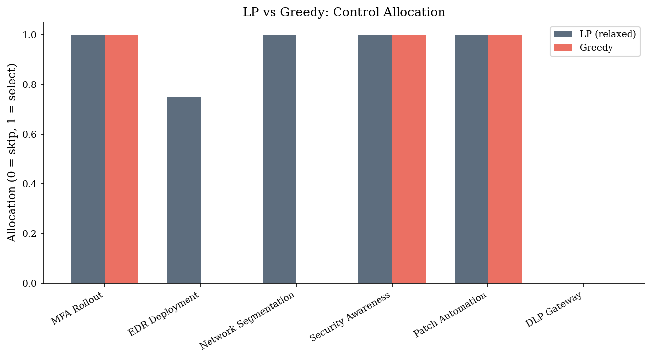
Allocation (1.0 = fully selected, fractional = partially):

MFA Rollout             1.0000
EDR Deployment          0.0000
Network Segmentation    0.7222
Security Awareness      1.0000
Patch Automation        1.0000
DLP Gateway             0.0000
dtype: float64

If the LP solution is all-integer, the greedy result is already optimal. A fractional entry indicates the LP needed to “split” a control to fill the budget exactly — the greedy approach either includes or excludes it. The gap between LP-relaxed and greedy tells you the cost of indivisibility.

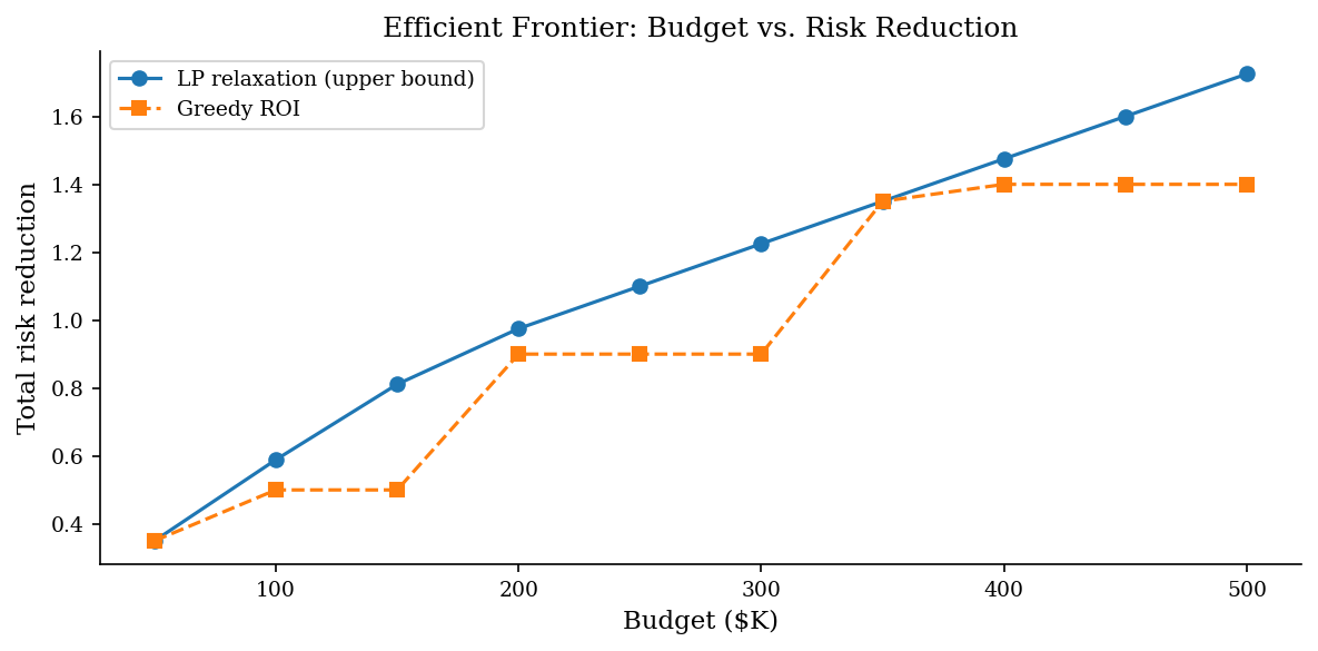
7 — Efficient Frontier: Budget vs. Risk Reduction

Varying the budget constraint and solving repeatedly traces an efficient frontier: the maximum achievable risk reduction at each budget level. This curve typically shows diminishing returns — the first \(500K buys substantially more risk reduction than the next \)500K — and provides a powerful communication tool for executive audiences.

The frontier answers two practical questions:

• Where does the curve flatten? Beyond this budget, you are buying increasingly marginal improvements. This is the natural “enough” point for budget negotiations.

• Are we on the frontier? If your current portfolio sits below the curve, you are leaving risk reduction on the table with the same spend. Reallocation beats new budget.

The frontier also answers questions that boards and CFOs routinely ask: “What is the marginal value of an additional $100K in security budget?” and “At what spending level do we hit diminishing returns?” Having a data-backed answer changes the conversation from “trust me” to “here is the trade-off curve.”

Any point below the frontier represents an inefficient allocation — you could get the same risk reduction for less money, or more reduction for the same money, by switching to a frontier portfolio. If your current control set falls well below the curve, that is a strong signal to reallocate before requesting additional budget.

budgets = np.arange(50_000, 500_001, 50_000)
lp_reductions = []
greedy_reductions = []

for b in budgets:
    # LP relaxation
    res = linprog(c_obj, A_ub=[costs], b_ub=[b], bounds=bounds, method="highs")
    lp_reductions.append(-res.fun if res.success else np.nan)

    # Greedy
    _, _, g_delta = select_controls_by_roi(deltas, costs, b)
    greedy_reductions.append(g_delta)

fig, ax = plt.subplots(figsize=(8, 4))
ax.plot(budgets / 1_000, lp_reductions, "o-", label="LP relaxation (upper bound)")
ax.plot(budgets / 1_000, greedy_reductions, "s--", label="Greedy ROI")
ax.set_xlabel("Budget ($K)")
ax.set_ylabel("Total risk reduction")
ax.set_title("Efficient Frontier: Budget vs. Risk Reduction")
ax.legend()
plt.tight_layout()
plt.show()

roi_vals = deltas / costs
order = np.argsort(roi_vals)[::-1]
bar_colors = [ACCENT if i in chosen_idx else VERY_LIGHT for i in order]

fig, ax = plt.subplots(figsize=(9, 5))
ax.barh([controls[i] for i in order],
        [roi_vals[i] for i in order],
        color=bar_colors, edgecolor='white')
ax.set_xlabel('ROI (Risk Reduction per Dollar)')
ax.set_title(f'Greedy Selection (red = selected, budget ${budget:,.0f})')
plt.tight_layout()
plt.show()

fig, ax = plt.subplots(figsize=(9, 5))
x_pos = np.arange(n)
width = 0.35

greedy_alloc = np.zeros(n)
for ci in chosen_idx:
    greedy_alloc[ci] = 1.0

ax.bar(x_pos - width/2, res.x, width, label='LP (relaxed)', color=DARK_BG, alpha=0.8)
ax.bar(x_pos + width/2, greedy_alloc, width, label='Greedy', color=ACCENT, alpha=0.8)
ax.set_xticks(x_pos)
ax.set_xticklabels(controls, rotation=30, ha='right')
ax.set_ylabel('Allocation (0 = skip, 1 = select)')
ax.set_title('LP vs Greedy: Control Allocation')
ax.legend()
plt.tight_layout()
plt.show()

Notice how the curve flattens: after a certain budget level, adding more money buys very little additional risk reduction. This is the classic diminishing-returns pattern and a powerful visual for communicating budget trade-offs to leadership. The gap between the LP relaxation (upper bound) and the greedy integer solution shows how much optimality the heuristic leaves on the table.

8 — Pitfalls

Weights must sum to 1. If they do not, the weighted score is on an arbitrary scale and comparisons across analyses become meaningless. Always normalize.

Incomparable scales. Cost in dollars and complexity on a 1–5 ordinal scale cannot be summed directly. Normalization (min-max, z-score, or rank-based) is mandatory before applying weights. The choice of normalization method itself affects results — document it.

Criteria washing. Adding redundant or highly correlated criteria inflates the importance of the dimension they represent. If “cost” and “TCO” are both included at equal weight, cost effectively gets double the influence. Each criterion should capture a distinct concern — audit your criteria for independence before you set weights.

Ignoring interactions. Both MCDA and greedy selection treat controls independently. In reality, deploying network segmentation changes the marginal value of east-west detection. Portfolio-aware methods (covered in later chapters) handle this, but for a first pass, independence is a reasonable simplifying assumption.

Optimizing the wrong objective. A technically optimal portfolio that ignores political feasibility, implementation sequencing, or organizational capacity will not survive contact with reality. Treat optimization output as a starting point for discussion, not a final answer.

Note: Both MCDA and LP are deterministic methods applied to uncertain inputs. The risk-reduction estimates, cost figures, and criteria scores feeding these models are themselves uncertain. Robust approaches — running the optimization across many Monte Carlo samples of the inputs — are covered in later chapters. For now, the key insight is that structured prioritization, even with imperfect inputs, consistently outperforms unstructured intuition.