Survival Analysis — Time-to-Event in Security

Security events have duration. Dwell time, time-to-patch, time-to-detect — these are all time-to-event problems, and they share a statistical structure that ordinary summary statistics handle poorly. Censoring is natural: some vulnerabilities are not patched by the end of an observation window, and dropping them biases every estimate. Means lie on right-skewed survival data even more than on loss data — the median from a Kaplan-Meier curve is almost always more honest.

For a full treatment of time-to-patch survival analysis applied to real vulnerability data, see Laura Voicu’s Elastic Security Labs article on time-to-patch metrics.

1 — Setup

import numpy as np
import matplotlib.pyplot as plt

from decision_security.synth import make_rng, survival_times
from decision_security.survival import km_estimator, nelson_aalen
from decision_security.viz import plot_km

rng = make_rng(42)

plt.rcParams.update({
    "font.family": "serif",
    "font.size": 10,
    "axes.labelsize": 11,
    "axes.titlesize": 12,
    "xtick.labelsize": 9,
    "ytick.labelsize": 9,
    "legend.fontsize": 9,
    "figure.dpi": 150,
    "axes.spines.top": False,
    "axes.spines.right": False,
})

PRIMARY = "#1A1A1A"
ACCENT = "#E74C3C"
DARK_BG = "#34495E"
LIGHT_GRAY = "#95A5A6"
MED_GRAY = "#7F8C8D"
VERY_LIGHT = "#BDC3C7"

2 — Generating Survival Data

We simulate 200 time-to-patch observations from a Weibull distribution (shape k=1.5, scale λ=30 days) with right-censoring at 60 days. Censoring means the vulnerability was still unpatched when we stopped watching.

times, events = survival_times("weibull", 200, rng=rng, k=1.5, lam=30, censor_at=60)

n_observed = int(events.sum())
n_censored = len(events) - n_observed
print(f"Observed (patched):   {n_observed}")
print(f"Censored (unpatched): {n_censored}")
print(f"Censoring rate:       {n_censored / len(events):.1%}")

Observed (patched):   193
Censored (unpatched): 7
Censoring rate:       3.5%

3 — Kaplan-Meier Curve

The Kaplan-Meier estimator gives a non-parametric estimate of the survival function S(t) — the probability that a vulnerability remains unpatched at time t. The horizontal line at S(t) = 0.5 marks the median survival time.

km_t, km_s = km_estimator(times, events)

fig, ax = plt.subplots(figsize=(8, 4))
plot_km(km_t, km_s, ax=ax)
ax.axhline(0.5, color=ACCENT, linestyle="--", linewidth=0.8, label="S(t) = 0.5")

median_idx = np.searchsorted(-np.array(km_s), -0.5)
median_time = km_t[median_idx]
ax.axvline(median_time, color=LIGHT_GRAY, linestyle=":", linewidth=0.8)
ax.set_xlabel("Days since disclosure")
ax.set_ylabel("S(t) — proportion unpatched")
ax.set_title("Kaplan-Meier: Time to Patch")
ax.legend()
plt.tight_layout()
plt.show()

print(f"50% of vulnerabilities are patched within {median_time:.0f} days.")

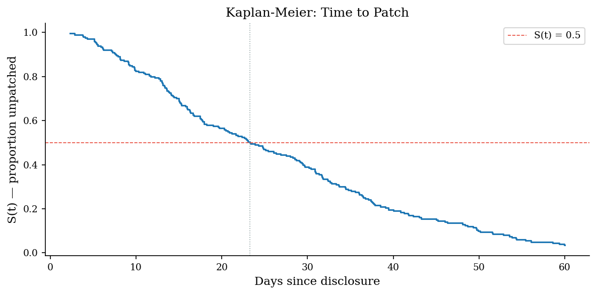
50% of vulnerabilities are patched within 23 days.

4 — Comparing Two Groups

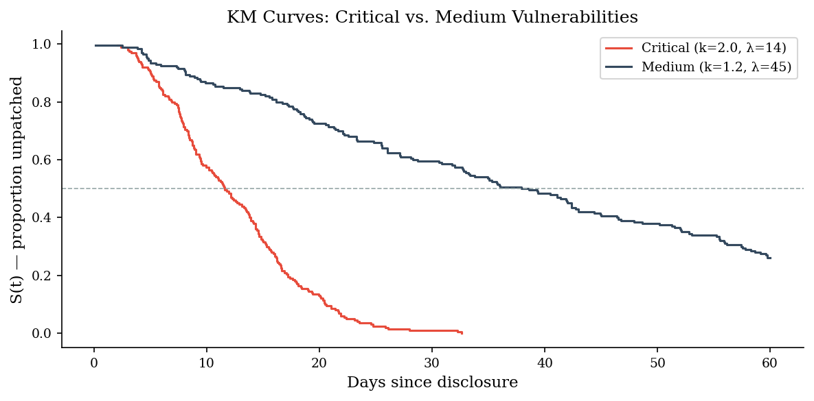
Risk-based patching prioritises critical vulnerabilities over medium ones. If the policy works, the two groups should have visibly different survival curves. Here we simulate “critical” (faster patching, k=2.0, λ=14) and “medium” (slower, k=1.2, λ=45) populations.

rng_crit = make_rng(42)
rng_med = make_rng(99)

t_crit, e_crit = survival_times("weibull", 200, rng=rng_crit, k=2.0, lam=14, censor_at=60)
t_med, e_med = survival_times("weibull", 200, rng=rng_med, k=1.2, lam=45, censor_at=60)

km_t_c, km_s_c = km_estimator(t_crit, e_crit)
km_t_m, km_s_m = km_estimator(t_med, e_med)

fig, ax = plt.subplots(figsize=(8, 4))
ax.step(km_t_c, km_s_c, where="post", color=ACCENT, label="Critical (k=2.0, λ=14)")
ax.step(km_t_m, km_s_m, where="post", color=DARK_BG, label="Medium (k=1.2, λ=45)")
ax.axhline(0.5, color=LIGHT_GRAY, linestyle="--", linewidth=0.8)
ax.set_xlabel("Days since disclosure")
ax.set_ylabel("S(t) — proportion unpatched")
ax.set_title("KM Curves: Critical vs. Medium Vulnerabilities")
ax.legend()
plt.tight_layout()
plt.show()

5 — Cumulative Hazard

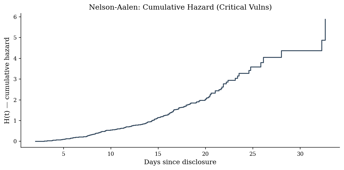
The Nelson-Aalen estimator gives the cumulative hazard H(t). The hazard rate is the instantaneous risk of the event at time t, given survival to t. An increasing slope means “the longer you wait, the worse it gets” — which is typical for critical vulnerabilities where exploits mature over time.

na_t, na_h = nelson_aalen(t_crit, e_crit)

fig, ax = plt.subplots(figsize=(8, 4))
ax.step(na_t, na_h, where="post", color=DARK_BG)
ax.set_xlabel("Days since disclosure")
ax.set_ylabel("H(t) — cumulative hazard")
ax.set_title("Nelson-Aalen: Cumulative Hazard (Critical Vulns)")
plt.tight_layout()
plt.show()

Pitfalls

• Censoring is information, not missing data. Dropping censored observations biases survival estimates upward — you are throwing away evidence that the event hadn’t happened yet, which makes everything look faster than it is.

• Median survival time is not the mean. Means are dragged by the right tail; the median is the time at which S(t) crosses 0.5. For right-skewed time-to-event data, the median is almost always the more useful summary.

• “Days since disclosure” is not “days of exposure.” Clock-start matters for time-to-patch metrics. A vulnerability disclosed publicly on day 0 may have been silently exploited for months. Survival analysis answers the question you ask it — make sure the clock measures what you actually care about.