Overdispersion – Testing the Poisson Assumption on Real Data#
Most cyber risk models count events with a Poisson distribution: one rate, events independent of each other, variance equal to the mean. Part 0 introduced the negative binomial as the alternative when counts vary more than that. This notebook does the test on real, public data and shows where the simple test misleads.
The data:
CISA Known Exploited Vulnerabilities (KEV) catalog – vulnerabilities CISA newly added to the catalog (with evidence of exploitation) per month, and the subset CISA marks as used in ransomware campaigns. A snapshot ships with the repository.
Ransomware.live – a public aggregator of ransomware leak-site postings, counted per month.
The causal lesson: a variable you did not model (here, a time trend) can produce the pattern you are testing for.
Setup#
import numpy as np
import pandas as pd
import matplotlib.pyplot as plt
from scipy import stats
import statsmodels.api as sm

from decision_security.synth import make_rng, sample
from _data import load_kev, ransomware_monthly_counts

rng = make_rng(42)

PRIMARY = "#1A1A1A"
ACCENT = "#E74C3C"
DARK_BG = "#34495E"
LIGHT_GRAY = "#95A5A6"

plt.rcParams.update({
    "font.family": "serif",
    "font.size": 10,
    "axes.labelsize": 11,
    "axes.titlesize": 12,
    "xtick.labelsize": 9,
    "ytick.labelsize": 9,
    "legend.fontsize": 9,
    "figure.dpi": 150,
    "axes.spines.top": False,
    "axes.spines.right": False,
    "text.color": PRIMARY,
    "axes.labelcolor": PRIMARY,
    "xtick.color": PRIMARY,
    "ytick.color": PRIMARY,
})

# Analysis window (inclusive, YYYY-MM)
START = "2025-06"
END = "2026-05"
REFRESH_KEV = False   # True: download the current KEV catalog instead of the snapshot

MONTHS = pd.period_range(START, END, freq="M")
print(f"{len(MONTHS)} months: {MONTHS[0]} to {MONTHS[-1]}")
12 months: 2025-06 to 2026-05
1. Data#
KEV entries are counted by the date CISA added them. Ransomware postings are counted by the month Ransomware.live assigns them (its monthly endpoint groups victims by attack date).
The KEV snapshot in data/kev_snapshot.csv keeps the notebook reproducible;
set REFRESH_KEV = True to use the current catalog. Both sources revise
their history, so a later run can give slightly different numbers.
About the Ransomware.live data. This notebook downloads it live from the anonymous v2 API (rate limited to 1 request per minute per endpoint) and caches it in
.cache/, so a first run takes about a minute per month; the raw data is never stored in this repository. The data is free for non-commercial use (personal research, academic, open source); for anything else, or for heavier use, see the terms and the PRO API. Do not republish the raw data, and credit “Source: Ransomware.live” with a link wherever you show it. Terms: https://www.ransomware.live/t&c
kev = load_kev(refresh=REFRESH_KEV)
kev["month"] = kev["dateAdded"].dt.to_period("M")
kev_all = kev.groupby("month").size().reindex(MONTHS, fill_value=0)
kev_rw = (kev[kev["knownRansomwareCampaignUse"] == "Known"]
          .groupby("month").size().reindex(MONTHS, fill_value=0))

# Cached in .cache/ (gitignored); the API is called only on a cold cache.
rw = ransomware_monthly_counts(MONTHS)

series = {
    "Ransomware leak-site postings": rw,
    "KEV CVEs added to the catalog": kev_all,
    "KEV ransomware-associated CVEs": kev_rw,
}
display(pd.DataFrame(series))
print("Leak-site postings source: Ransomware.live (https://www.ransomware.live)")
| Ransomware leak-site postings | KEV CVEs added to the catalog | KEV ransomware-associated CVEs | |
|---|---|---|---|
| 2025-06 | 549 | 20 | 1 |
| 2025-07 | 500 | 20 | 4 |
| 2025-08 | 528 | 15 | 1 |
| 2025-09 | 556 | 16 | 1 |
| 2025-10 | 791 | 31 | 3 |
| 2025-11 | 707 | 11 | 0 |
| 2025-12 | 761 | 20 | 2 |
| 2026-01 | 732 | 17 | 2 |
| 2026-02 | 784 | 28 | 2 |
| 2026-03 | 814 | 26 | 2 |
| 2026-04 | 791 | 31 | 9 |
| 2026-05 | 766 | 21 | 3 |
Leak-site postings source: Ransomware.live (https://www.ransomware.live)
2. The Simple Test: Variance-to-Mean Ratio#
For a Poisson process the variance equals the mean, so the variance-to-mean ratio (VMR, the index of dispersion) is 1. The dispersion test compares \((n-1)\cdot\text{VMR}\) with a \(\chi^2_{n-1}\) distribution; a small p-value means the counts vary more than Poisson allows.
def dispersion(counts):
    x = np.asarray(counts, dtype=float)
    n, mean, var = len(x), x.mean(), x.var(ddof=1)
    vmr = var / mean
    p = stats.chi2.sf((n - 1) * vmr, n - 1)
    return {"n": n, "mean": mean, "variance": var, "VMR": vmr, "p (Poisson)": p}


raw = pd.DataFrame({k: dispersion(v) for k, v in series.items()}).T
raw.round({"mean": 1, "variance": 1, "VMR": 2, "p (Poisson)": 4})
| n | mean | variance | VMR | p (Poisson) | |
|---|---|---|---|---|---|
| Ransomware leak-site postings | 12.0 | 689.9 | 14333.2 | 20.78 | 0.0000 |
| KEV CVEs added to the catalog | 12.0 | 21.3 | 41.2 | 1.93 | 0.0312 |
| KEV ransomware-associated CVEs | 12.0 | 2.5 | 5.4 | 2.15 | 0.0145 |
3. The Trap: Trend Looks Like Clustering#
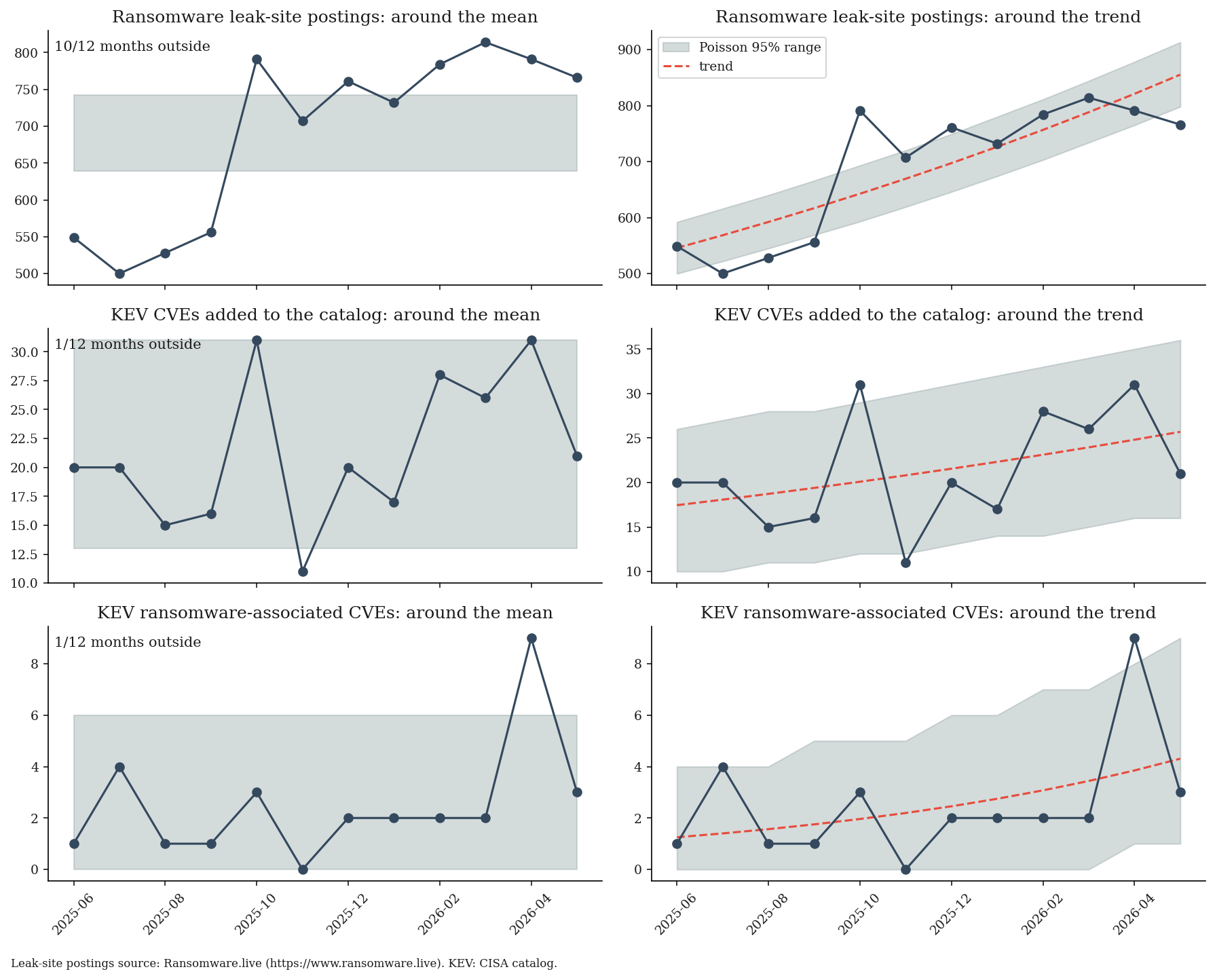
A growing series inflates the variance around its overall mean even if arrivals around the trend are perfectly regular. The trend is an omitted variable: leave it out and the test attributes its effect to clustering.
To separate the two, fit a Poisson regression with a time trend (log link) and measure the dispersion that is left: the Pearson \(\chi^2\) divided by its degrees of freedom. Values near 1 mean “Poisson around the trend”. The log-linear trend is itself an assumption; the last check below replaces it with one level shift.
The negative binomial shape \(k\) (the same \(k\) as in Part 0; many texts call it \(r\)) is then estimated two ways:
raw: method of moments on the counts, \(k = \text{mean}^2 / (\text{variance} - \text{mean})\);
detrended: a negative binomial (NB2) regression with the same time trend, \(k = 1/\alpha\).
Higher \(k\) means the rate varies less (closer to Poisson). \(k\) measures rate variability, so it compares across series; the VMR it produces depends on the mean (VMR = 1 + mean/\(k\)).
def detrended(counts):
    y = np.asarray(counts, dtype=float)
    t = np.arange(len(y))
    X = sm.add_constant(t)
    pois = sm.GLM(y, X, family=sm.families.Poisson()).fit()
    df = len(y) - X.shape[1]
    mean, var = y.mean(), y.var(ddof=1)
    k_raw = mean**2 / (var - mean) if var > mean else np.inf
    try:
        nb = sm.NegativeBinomial(y, X, loglike_method="nb2").fit(disp=0)
        alpha = nb.params[-1]
        k_det = 1 / alpha if alpha > 1e-8 else np.inf
    except Exception:
        k_det = np.nan
    return {"trend per month": np.exp(pois.params[1]) - 1,
            "dispersion after trend": pois.pearson_chi2 / df,
            "p (Poisson around trend)": stats.chi2.sf(pois.pearson_chi2, df),
            "NB shape k (raw)": k_raw,
            "NB shape k (detrended)": k_det}


det = pd.DataFrame({k: detrended(v) for k, v in series.items()}).T
det.style.format({"trend per month": "{:+.1%}", "dispersion after trend": "{:.2f}",
                  "p (Poisson around trend)": "{:.4f}", "NB shape k (raw)": "{:.1f}",
                  "NB shape k (detrended)": "{:.1f}"})
| trend per month | dispersion after trend | p (Poisson around trend) | NB shape k (raw) | NB shape k (detrended) | |
|---|---|---|---|---|---|
| Ransomware leak-site postings | +4.2% | 7.57 | 0.0000 | 34.9 | 129.7 |
| KEV CVEs added to the catalog | +3.6% | 1.74 | 0.0650 | 23.0 | 46.4 |
| KEV ransomware-associated CVEs | +11.9% | 1.67 | 0.0811 | 2.2 | 7.6 |
for name in series:
    print(f"{name}:")
    print(f"  VMR {raw.loc[name, 'VMR']:.2f} -> dispersion after trend "
          f"{det.loc[name, 'dispersion after trend']:.2f}   "
          f"(p around trend = {det.loc[name, 'p (Poisson around trend)']:.3f})")

# Same series, one level shift instead of a trend, placed at the largest month-to-month jump
y = rw.values.astype(float)
step = int(np.argmax(np.abs(np.diff(y)))) + 1
X_step = sm.add_constant((np.arange(len(y)) >= step).astype(float))
shift = sm.GLM(y, X_step, family=sm.families.Poisson()).fit()
print(f"\nRansomware leak-site postings: dispersion after trend "
      f"{det.loc['Ransomware leak-site postings', 'dispersion after trend']:.2f} -> "
      f"after a level shift at {MONTHS[step]} {shift.pearson_chi2 / shift.df_resid:.2f}")
Ransomware leak-site postings:
  VMR 20.78 -> dispersion after trend 7.57   (p around trend = 0.000)
KEV CVEs added to the catalog:
  VMR 1.93 -> dispersion after trend 1.74   (p around trend = 0.065)
KEV ransomware-associated CVEs:
  VMR 2.15 -> dispersion after trend 1.67   (p around trend = 0.081)

Ransomware leak-site postings: dispersion after trend 7.57 -> after a level shift at 2025-10 1.46
4. What It Looks Like#
Grey band: the 95% range a Poisson process would produce.
fig, axes = plt.subplots(len(series), 2, figsize=(12, 3.2 * len(series)), sharex=True)
x = np.arange(len(MONTHS))
labels = [str(m) for m in MONTHS]
for row, (name, s) in zip(axes, series.items()):
    y = s.values.astype(float)
    lo, hi = stats.poisson.ppf([0.025, 0.975], y.mean())
    row[0].fill_between(x, lo, hi, color=LIGHT_GRAY, alpha=0.4, label="Poisson 95% range")
    row[0].plot(x, y, "o-", color=DARK_BG)
    row[0].set_title(f"{name}: around the mean")
    outside = int(((y < lo) | (y > hi)).sum())
    row[0].text(0.01, 0.92, f"{outside}/{len(y)} months outside", transform=row[0].transAxes)
    fit = sm.GLM(y, sm.add_constant(x), family=sm.families.Poisson()).fit()
    mu = fit.fittedvalues
    row[1].fill_between(x, stats.poisson.ppf(0.025, mu), stats.poisson.ppf(0.975, mu),
                        color=LIGHT_GRAY, alpha=0.4, label="Poisson 95% range")
    row[1].plot(x, mu, "--", color=ACCENT, label="trend")
    row[1].plot(x, y, "o-", color=DARK_BG)
    row[1].set_title(f"{name}: around the trend")
for ax in axes[-1]:
    ax.set_xticks(x[::2])
    ax.set_xticklabels(labels[::2], rotation=45)
axes[0][1].legend(loc="upper left")
fig.text(0.01, 0.005, "Leak-site postings source: Ransomware.live (https://www.ransomware.live). "
         "KEV: CISA catalog.", fontsize=8)
plt.tight_layout(rect=(0, 0.02, 1, 1))
plt.show()
5. Why It Matters for a Risk Model#
Same average rate, different clustering. The negative binomial is a Poisson process whose rate itself varies: each year the rate is drawn from a Gamma distribution with shape \(k\) and mean equal to the long-run rate. Large \(k\) recovers Poisson; small \(k\) means some years are much worse than others.
Note: this is not the same as a Gamma distribution for the time between events. For inter-arrival times, shape 1 is Poisson, shape above 1 is more regular than Poisson, and only shape below 1 clusters.
RATE = 3.0          # expected events per year for one organisation (illustrative)
YEARS = 200_000

sims = {
    "Poisson": sample("poisson", YEARS, rng=rng, lam=RATE),
    "Negative binomial, k = 30 (mild clustering)": sample("negbin", YEARS, rng=rng, mean=RATE, k=30),
    "Negative binomial, k = 2 (strong clustering)": sample("negbin", YEARS, rng=rng, mean=RATE, k=2),
}
table = pd.DataFrame({name: {"mean": v.mean(), "P(0 events)": (v == 0).mean(),
                             "P(>= 6 events)": (v >= 6).mean(), "P(>= 8 events)": (v >= 8).mean()}
                      for name, v in sims.items()}).T
table.round(3)
| mean | P(0 events) | P(>= 6 events) | P(>= 8 events) | |
|---|---|---|---|---|
| Poisson | 2.998 | 0.050 | 0.083 | 0.012 |
| Negative binomial, k = 30 (mild clustering) | 3.008 | 0.056 | 0.094 | 0.017 |
| Negative binomial, k = 2 (strong clustering) | 2.995 | 0.159 | 0.158 | 0.070 |
Clustered arrivals produce more quiet years and more bad ones. If counts are clustered, a model that assumes Poisson understates the right tail of the loss exceedance curve.
6. Pitfalls#
A high VMR is not proof of clustering. Remove the trend before reading the VMR as burstiness, and keep the raw estimate only as a sensitivity case.
Global series measure common shocks, not your organisation. Once the trend is removed, what is left can come from a trend of the wrong shape (a level shift, or a change in the source’s coverage), from common shocks (a campaign wave or mass-exploited vulnerability raising many organisations’ rates at once) and from batching (one campaign, many victims). For the ransomware series most of the remaining dispersion is a level shift in October 2025 (1.46 against 7.57; the step month is picked from the data, which favours it), not month-to-month clustering. Differences between organisations don’t show up in a global time series, and burstiness specific to one organisation averages out. An organisation can measure its own burstiness from its telemetry, if events are frequent enough to count.
Know what is counted. Leak-site postings are (mostly) claimed victims of successful attacks who did not pay, closer to loss events than threat events; some claims are recycled or fake. KEV entries count vulnerabilities CISA newly added to the catalog (with evidence of exploitation), not attacks and not the date exploitation started. Neither is an individual attempt, so the parameters describe successful attacks and catalog additions.
Twelve points is little data. The tests have little power on 12 months. Both KEV series stay above Part 0’s 1.5 rule of thumb after detrending (1.74 and 1.67), yet the test cannot reject Poisson: a non-rejection is not proof of Poisson.
Public sources are revised. Both sources change their history and have their own coverage gaps. KEV’s ransomware flag is updated after the fact, so recent months undercount ransomware-associated CVEs. Treat the parameters as a range for sensitivity analysis, not as point values.
Data: CISA KEV catalog (public domain). Source: Ransomware.live (free for non-commercial use; https://www.ransomware.live/t&c).